I never thought that this series would grow to this length - but the more I learn about this topic, the more I find things to write about. Starting from what seemed like a very trivial sketch - some circles bouncing around on the canvas - I actually ended up learning so much about simulating physics, about collision detection, optimizations for computing collisions faster, how springs work, how to connect particles with springs and create meshes, and even taking a dip into soft body physics.
And now, what if I told you that there was a completely different approach to doing all of these things? That the way we implemented our particle system in it's current state, was just one of the different approaches in which things can be done? And that the system we created is actually flawed in many ways? Yes, there's actually many issues that still remain and that we're going to tackle throughout this article.
First we'll go over what we've done so far, again, but this time around examine it from a mathematical point of view. And while we're at it, we'll also identify some problems that exist in this system. In the second part of this article we'll then talk about Verlet Integration, a different numerical method to compute the movement of particles on the canvas.
It might seem like a scary term at first, but it's actually not that complicated, it just requires us to do a little bit of setup to get there. Overall, it isn't even very difficult to implement. One important aspect of Verlet Integration is it's numerical stability - we'll see what that means towards the end of the article - making it excellent for scenarios where we have a number of interconnected particles: for instance when we're trying to model soft body physics! That's why it's worth looking into, to help us and make our future soft body simulations more accurate, more robust and overall much smoother!
Another thing, before we start - I want to give a gigantic shoutout to this amazing video from Gustavo, who creates educative computer science and game dev content on the Pikuma Youtube channel. I genuinely don't know why it's only got roughly 10k views, it deserves many more.
It's a bit of long watch, but really worth it. I learned a lot from it. Thank you Gustavo!
Gustavo explains all of the concepts that we're also gonna tackle so beautifully and in the very best order that they could be explained - starting with the Regular Euler Integration approach and then moving on towards Verlet Integration. I definitely recommend watching it, it helped me understand things a lot better. Also go follow Pikuma on Twitter for more content like this!
That said, let's get into the tutorial 👇
Euler Integration
Let's have a look at how we've computed the movement of particles in our system, so far.
Essentially, the future position of a particle on the canvas, can be determined by means of it's current position, it's velocity and an acceleration term, in addition to other forces that act upon the velocity in a similar manner to the acceleration. I go over what velocity and acceleration are in this post if you're not up to speed:
But to recap, the velocity of a particle is a vector that indicates the direction that it is moving in, as well as the speed that it is moving at. The acceleration is a term that indicates how the velocity is changing over time. If we're speeding up, or slowing down basically. The new position of a particle is calculated by adding the velocity vector to it's current position. The formula that describes this is simply the addition of the two vectors:
\( P_{n+1} = P_{n} + V_{n} \)
Similarly, velocity is defined in terms of acceleration - the new velocity becomes the current velocity plus the acceleration vector:
\( V_{n+1} = V_{n} + a_{n} \)
If you're like me and can understand this better as code, it would look as follows:
position.x = position.x + velocity.x
position.y = position.y + velocity.y

velocity.x = velocity.x + acceleration.x
velocity.y = velocity.y + acceleration.y
In p5js, the wonderful framework that we use to visualize things, we have the convenient vector class that makes things a bit easier, and cuts the number of lines of code that we have to write in two:
position = p5.Vector.add(position, velocity)
velocity = p5.Vector.add(velocity, acceleration)
This way of computing the future position of a particle is called Euler Integration! It is one of the simplest ways to compute the movement of particles on the canvas, and is also very often used for video games, because of it's simplicity. With just a few lines of code we can make particles move around on the canvas!
The Problem with Euler Integration
But what are we actually doing here? Why is it called Euler Integration? What are we integrating after all?
As the video by Gustavo illustrates so beautifully, a particle moving in space is actually a continuous phenomenon - computers however, are discrete machines. We can only represent continuous phenomenons as discrete approximations. A particle moving through space from point A to point B, actually physically moves from point A to B, occupying all of the space that lies between these two points as time passes. Just like a puck gliding over an air hockey table.
In our Javascript simulation, the particle doesn't behave like that though. The particle jumps forward in incremental and discrete steps towards it's destination. We are updating it's position by addition of a velocity vector, a discrete quantity, after all. We only perceive this as a smooth motion because these steps are generally minuscule, obfuscating the fact that they're discrete steps and creating the illusion of a smooth motion.
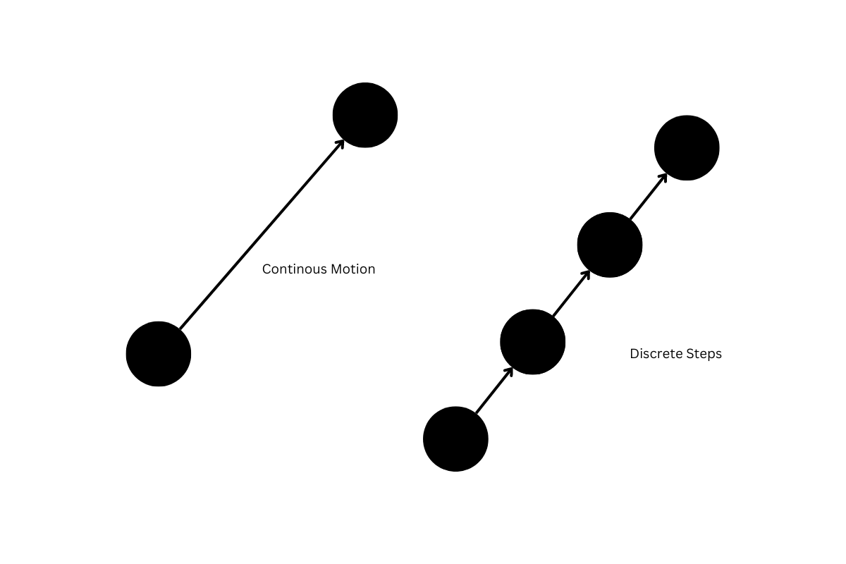
To put it simply, approximating a continuous function with discrete numeric steps, is usually known as integration.
An since it's only an approximation, a problem arises: an error gradually accumulates over time. This error can sometimes become more and more apparent the longer we let our particle simulation run. This might not be a big deal when it comes to creative coding and generative art, where we usually aim to make a chaotic and fun-to-watch particle chaos, but in other scenarios this is problematic.
Let's see why this is, and demonstrate it with a simple sketch - let this run for a while and observe the behavior of the particles:
What is happening here? Why does the particle keep bouncing higher and higher over time? Euler Integration is a method that gains energy over time. This is due to the approximation error that arises: every time that we calculate the new position of the particle, we're actually overshooting the actual real value by a little bit leading to an offset. This manifests itself by the particle bouncing higher and higher over time. And this isn't ideal, we don't want things to get more volatile over time.
Semi-implicit Euler Integration
There's actually a hack to make this system lose energy over time instead. In fact it's what we've been doing all along in the previous versions of our particle system! Let me explain!
In the previous tutorials, we would add forces directly to the particle's velocity, such as the particle's acceleration and gravity. This is technically correct, but not exactly the proper way of doing things.
Normally, in Euler integration, all external forces are first combined, for instance the gravitational force, and then used to determine the acceleration of the particle. The acceleration being the sum of the external forces, divided by the mass of the particle. This resulting acceleration can then be added on to the current velocity, to determine the future velocity, which in turn lets us compute the new position of the particle. These steps essentially constitute the update() function of the particle, and would look as follows:
update(sumOfForces){
  this.acceleration = p5.Vector.div(sumOfForces / this.mass)

  this.position = p5.Vector.add(this.position, this.velocity)
  this.velocity = p5.Vector.add(this.velocity, this.acceleration)
}
An exactly in this order! Order is important!
Note that the new position of the particle is computed before we update it's velocity. This is the proper order of computations in the Euler integration method. Doing things in this manner however, will lead to an accumulating error that makes particles gain energy over time as we mentioned before - and is reflected by an ever increasing velocity, which in turn makes the particle speed up more and more over time.
Have a look at this example that demonstrates two different approaches, where the first particle on the left, uses the exact update function as shown above, using the proper Euler integration method. The second particle on the right, is updated in the same manner as in the preceding tutorials, where we update the velocity with a seperate addForce() function - that adds external forces directly to the particle's velocity. We observe two very different behaviors:
But wait a second, there aren't really any external forces applied to the particles, other than the gravity vector that we've initialized at the beginning of the setup function. So why does the second particle keep bouncing in place, and doesn't exhibit any increase in height over time, like the first one?
It's due to the order of operations. We've essentially flipped the order of the velocity update and the position update, computing the new velocity of the particle before we compute it's new position. This ends up being the semi-implicit Euler method, and results in a particle behavior that doesn't gain energy over time - in fact, it does the opposite, the accumulated error leads to an undershooting of the actual position of the particle, losing energy over time.
Therefore, if we were to flip these two lines in the draw loop, we'd obtain the same behavior of the regular Euler method, and the particle would also end up gaining height over time:
ourParticle.addForce(gravity)
ourParticle.update()
Here, same code, just the two lines of code flipped:
Even though we did inadvertently end up implementing the semi-implicit approach, it's always better to write things in a clear and readable manner. The update function for a particle that implements the semi-implicit Euler method would look as follows:
update(sumOfForces){
  this.acceleration = p5.Vector.div(sumOfForces / this.mass)

  this.velocity = p5.Vector.add(this.velocity, this.acceleration)
  this.position = p5.Vector.add(this.position, this.velocity)
}
Computation of position and velocity have a different order now.
Simply placing the velocity update before the position update. Hence, the order of things matters a lot! Here's the same example again, but rewritten in a nicer way:
...
Hold up a sec! If the semi-implicit Euler method should be losing energy over time, why does the second particle maintain the same bounce height?
A Clarification on our previous Implementation
Well, that's actually because this is a very special case of the semi implicit Euler method: when the initial velocity of a particle is a zero vector, then it will actually not lose energy over time and end up conserving it. We'll actually exactly hit the mark and have the particle bounce up to it's original height every time.
Have a look at this example, where we pass in a random vector as the particle's initial velocity as we create it, it will actually bounce lower and lower, and after a while come to a full stop:
Phew, glad we solved this mystery! The reasons why an initial zero velocity leads to conservation of energy are a bit more elaborate, but I'm just going to side step that for now! I looked into it a bit, and it seems that in this special case the particle ends up being a Hamiltonian system, which is essentially a special kind of system that conserves it's energy as already mentioned.
And just to make sure that things are clear:
It's important to understand that in the particle systems that we've programmed previously, it might have seemed that we did things correctly, but you'd notice that if we were to let things run long enough, everything would eventually end up coming to a standstill. This can end up being a bit confusing, hence I really recommend playing with the formulas for yourself, and trying to recreate the simple bouncing particle sketches from scratch to get a feel for this.
Why am I bringing this up? Because I don't want you to mistake the previous sketches for accurate physics simulations, where it might've seemed that we've created a realistic gravitational pull directed towards the bottom of the canvas. This is in fact not what is actually happening.
In a friction-less world, a ball would keep bouncing forever. In our case the particle didn't stop bouncing because of friction though - we didn't implement any friction - it stops bouncing merely because it was losing energy due to the integration method that we were using, causing an accumulating error. I hope this makes sense. It felt necessary to clarify this, to be able to move forward with a better understanding of what we are actually doing.
Updating our system with a time-step component
Up until this point, the little physics simulations that we've created have an apparent animation speed that is directly tied to the frame rate of the draw loop. Increasing this frame rate, would also lead to an increase in the speed of the animation, and vice versa. And this isn't ideal, we'd much rather have the speed of the engine be independent from the frame rate.
For instance if we run the previous sketches at 30 frames per second, rather than 60 frames per second, then the simulations would only progress half as fast. So, how do we solve this and make the speed of the simulation independent from the frame rate?
Well, there's actually another variable that goes into the formulas for computing the position and velocity of a particle in movement. Delta Time: a time increment that scales the acceleration and velocity in the velocity and position update statements respectively. This time increment variable usually represents the time elapsed since the beginning of the previous frame and the beginning of the current frame. Essentially the formulas then become:
\( P_{n+1} = P_{n} + V_{n} * \Delta t \)
\( V_{n+1} = V_{n} + a_{n} * \Delta t \)
This scaling ensures that the simulation progresses at a consistent rate, regardless of the frame rate.
P5 already provides this delta time variable out of the box in milliseconds, and we'd simply have to scale it, dividing it by a factor of 1000:
let dt = deltaTime / 1000

particle.update(sumOfForces, dt)
Then we can simply pass it in as another input to the particle's update function.
And in action this would look as follows, for instance here's a sketch at the native frame rate:
And here's the same sketch at a very choppy 10 fps:
Note here that we had to make some changes to the overall numbers, for instance we reduced the mass of the particle and cranked the force of the gravity, otherwise things would overall be very slow.
And that concludes everything I want to say about Euler Integration, I think that we're ready to tackle Verlet Integration now!
Verlet Integration
If you've got a solid grasp on everything that preceded then the rest should be a walk in the park!

In a nutshell, Verlet Integration is a different approach to computing the future position of a moving particle, without us requiring to explicitely store the velocity of that particle. Yes, that's right, with Verlet Integration we can do without the velocity variable, because we can actually estimate with a nifty formula - in which we only need to remember the previous position of the particle. We'll deduce this formula from the semi-implicit form that we had a look at earlier.
So instead of explicitly storing the velocity of the particle and manipulating it, we'll now store the current position of the particle, it's previous position as well as it's acceleration. Let's see how this works!
Backtracking a bit, and returning to the formulas for the semi-implicit Euler Integration method, we have:
\( V_{n+1} = V_{n} + a_{n} * \Delta t \)
\( P_{n+1} = P_{n} + V_{n+1} * \Delta t \)
Note how in the semi-implicit form the new position depends on the new velocity. These same position update formula, for the previous position of the particle would look as follows - simply going back one step in time, as indicated by the suffixes of the variables:
\( P_{n} = P_{n-1} + V_{n} * \Delta t \)
We can rewrite this in terms of the current and previous position:
\( V_{n} = \frac{P_{n} - P_{n-1}}{\Delta t} \)
This means that the current velocity can actually be deduced from the old and the current position. Ok, this is great! How does that help us find the next position of the particle though? Let's rewrite the formula for the next position, substituting the \( V_{n+1} \) term:
\( P_{n+1} = P_{n} + ( V_{n} + a_{n} * \Delta t ) * \Delta t \)
And from before we know that \( V_{n} \) can be written in terms of the old and previous position, hence we'd obtain the following:
\( P_{n+1} = P_{n} + ( \frac{P_{n} - P_{n-1}}{\Delta t} + a_{n} * \Delta t ) * \Delta t \)
Let's clean this up a bit and we get:
\( P_{n+1} = P_{n} + P_{n} - P_{n-1} + a_{n} * \Delta t^2 \)
And more concisely:
\( P_{n+1} = 2P_{n} - P_{n-1} + a_{n} * \Delta t^2 \)
And as you can see, this formula doesn't require any velocity term for the computation of the next position of the particle!
Implementing a Verlet Particle
The hard part's done - armed with this new formula we can now implement our Verlet Particle. First, let's add a member variable in which we'll store the old position:
class Particle{
  constructor(position){
    this.position = position

    // initially we'll set the old position to the current position
    this.oldPosition = this.position

    // we can also pass this in as an input
    this.mass = 1
    this.radius = 15
  }
}
As for the update function, we'll now implement Verlet integration:
update(sumOfForces, dt){
  this.tempPosition = this.position

  this.position = p5.Vector.add(p5.Vector.sub(p5.Vector.mult(this.position, 2),
    this.oldPosition), p5.Vector.mult(sumOfForces, dt*dt))

  this.oldPosition = this.tempPosition
}
Here we need to first store the current position in a temporary variable, since it will become the old position after we've computed the new current position. Then we have a gnarly line in which we simply apply the formula that we concluded with in the previous section to compute the new position of the particle, and finally we set the old position to the temporary value that we stored earlier.
Boundary Checks with Verlet Integration
So we have one little problem left when it comes to checking if the particle is within the bounds of the canvas. Previously we'd simply point the velocity of the particle into the opposite direction when we hit a canvas boundary.
Now we don't have an explicit velocity vector anymore and can't use that exact method anymore to make our particles bounce off of the boundaries. But we can sidestep this by computing the velocity temporarily, by subtracting the old position from the current position and then using that velocity to cheat a little bit. We'll essentially reflect the old position around the current position of the particle, in a way pretending that we are coming from beyond the canvas boundary.
And that would look as follows:
constrain(){
  let velocity = p5.Vector.sub(this.position, this.oldPosition)

  if(this.position.x < 0){
    this.position.x = 0
    this.oldPosition.x = this.position.x + velocity.x
  }else if(this.position.x > 400){
    this.position.x = 400
    this.oldPosition.x = this.position.x + velocity.x
  }else if(this.position.y < 0){
    this.position.y = 0
    this.oldPosition.y = this.position.y + velocity.y
  }else if(this.position.y > 400){
    this.position.y = 400
    this.oldPosition.y = this.position.y + velocity.y
  }
}
And in action our final Verlet simulation:
You can see here that Verlet Integration also suffers from a loss of energy over time, but maybe not as harshly as the semi-implicit Euler Integration method.
Numerical Stability
At the very start of this article, I mentioned that Verlet Integration is numerically more stable than Euler Integration. Let's put this to the test and compare the two methods - let's see how quickly the two lose energy in comparison to each other:
Well it seems that there isn't much difference here really. Bummer.
But wait, we're not actually doing this the right way! This energy loss and the accumulating error have a lot to do with the size of the time increment. The larger this time increment, the quicker this accumulated error will become apparent. That means if we were to make this time step smaller, we'd be able to make more accurate predictions. How do we do this though?
We simply run our simulation several times per frame, dividing the time increment by the number of simulation steps. Let's compare the methods again - but this time let's run the update step 10 times every frame, the draw loop would look as follows now:
function draw() {
  background(220);

  let dt = deltaTime/1000

  for(let n = 0; n < 10; n++){
    verletP.update(gravity, dt/10)
    verletP.constrain()


    eulerP.semiImplicitUpdate(gravity, dt/10)
    eulerP.constrain()
  }

  verletP.display()
  eulerP.display()


  line(0, 200, 400, 200)
}
And in action:
Here I also give the Euler particle a random starting velocity to give the Verlet particle a fair chance, because the Euler particle would simply bounce forever if it's initial velocity is zero as mentioned before. In this scenario you can see that Verlet integration conserves energy much, much better than the Euler method!
In both cases, this means that our simulation will be more accurate for more time steps, but comes at the expense of a computational overhead. Ultimately it will boil down to your application and how accurate you need/want things to be!
Concluding Thoughts
In this article we covered Verlet Integration, and also extensively discussed the regular Euler Integration method that is most commonly used for simulating simple particle system, as well as other applications. We also discussed some of the problems with it, such as the accumulating error that leads to a gain or loss of energy over time and discussed how to make things more accurate by running the simulation over smaller time steps.
In the next post we'll discuss how to do collisions and springs with the Verlet integration method and then also revisit soft body physics.
As always, I hope you enjoyed this post, I definitely had a lot of fun writing it. If you did, consider sharing it on your socials, or signing up to the newsletter to get updates whenever new content is posted on the blog. It helps a lot! Otherwise, cheers and happy sketching ~ Gorilla Sun 🌸